Environment-dependent TB#
Method Introduction:#
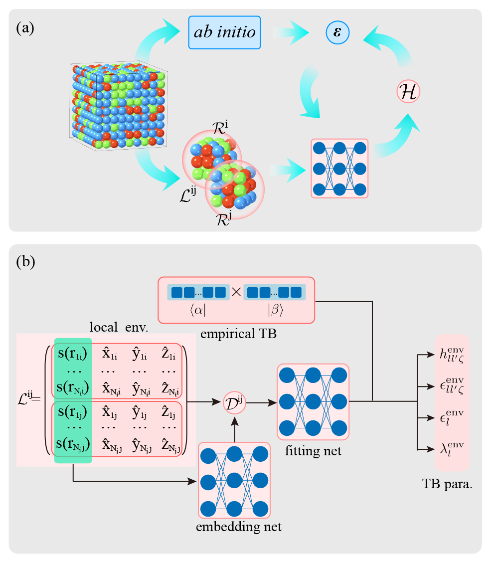
The basic idea of the DeePTB method is to fit the DFT electronic band structure through deep learning, thereby constructing a TB model to achieve first-principles accuracy.
In the TB model, the Hamiltonian matrix elements can be expressed as:
where \(i\), \(j\) are site indices. \(l\) and \(m\) are angular and magnetic quantum numbers. \(H\) is the Hamiltonian operator. In DeePTB, we choose the traditional Slater-Koster (SK) parameterized Hamiltonian, where all the Hamiltonian can be expressed in terms of SK integrals: \(h_{ss\sigma}, h_{sp\sigma}, h_{pp\sigma}, h_{pp\pi}, \cdots\), etc. Based on these SK integrals, we can construct Hamiltonian matrix as follows:
Here, \(\mathcal{U}_{\zeta}\) is a \([2l+1,2l^\prime+1]\) matrix, and \(\zeta\) represents the key type, such as \(\sigma, \pi\), etc. The specific form of \(\mathcal{U}_{\zeta}\) can be found in Ref:1.In traditional SK-TB, SK integrals often use analytical expressions based on the following empirical rules, and are based on the two-center approximation.
In DeePTB, we use a neural network-based method to predict SK integrals, which is expressed as:
where \(h_{ll^\prime{\zeta}}\) is also an SK integral based on an analytical expression. In DeePTB, the undetermined coefficients of the analytical expression are represented by neurons. \(h^{\text{env}}_{ll^\prime{\zeta}}\) depends on the local environment introduced by the neural network. Refer to DeePTB paper for more information.
In the following, we will use Silicon as an example to show the full training procedure of DeePTB.
Example: Bulk Silicon#
Bulk silicon has diamond structure at room temperature and pressure. Due to its widespread applications in the semiconductor industry, it has been a significant important element in modern society. Here we provide an example of building a silicon DeePTB model. By following this instruction step-by-step, you will be introduced to the high-level functionalities of DeePTB, which can provide a model bypass empirical TB, to achieve ab initio accuracy.
This example can be seen in the example/silicon folder. The whole training procedure can be summarized as below:
This procedure contains the full steps to training an environmentally corrected DeePTB model. The converged model can predict the electronic structure of both perfect crystals and the configurations with atomic distortion, while can generalize to structures with more atoms.
1. Data Preparation#
The data for training and plotting contains in data folders:
deeptb/examples/silicon/data/
|-- kpath.0                 # train data of primary cell. (k-path bands)
|-- kpathmd25.0             # train data of 10 MD snapshots at T=25K   (k-path bands)
|-- kpathmd100.0            # train data of 10 MD snapshots at T=100K  (k-path bands)
|-- kpathmd300.0            # train data of 10 MD snapshots at T=300K  (k-path bands)
|-- kpt.0                   # kmesh samples of primary cell  (k-mesh bands)
|-- kpath_spk.0
|-- silicon.vasp            # structure of primary cell
Each of these folders, contains data files with required format, here we give an examples of kpath.0:
deeptb/examples/silicon/data/kpath.0/
-- info.json
-- eigs.npy
-- kpoints.npy
-- xdat.traj
The meaning and useage of the files can refer to ../quick_start/input.md.
2. Training Neural Network Emperical TB Model (no env)#
2.1 Training a First Nearest Neighbour Model#
We first analyse the bond length by running.
dptb bond ./data/silicon.vasp
The output will be like:
 Bond Type         1         2         3         4         5
------------------------------------------------------------------------
     Si-Si      2.35      3.84      4.50      5.43      5.92
The fitting of empirical TB on the first nearest neighbours shares the same procedure as the hBN example. We suggest the user try on hBN before proceeding. This time, the training starts from the first nearest neighbour checkpoint in input folder. Run the following command to train the first nnsk model:
dptb train ./input/2-1_input.json -o ./nnsk
2.2 Add More Orbitals and Neighbours#
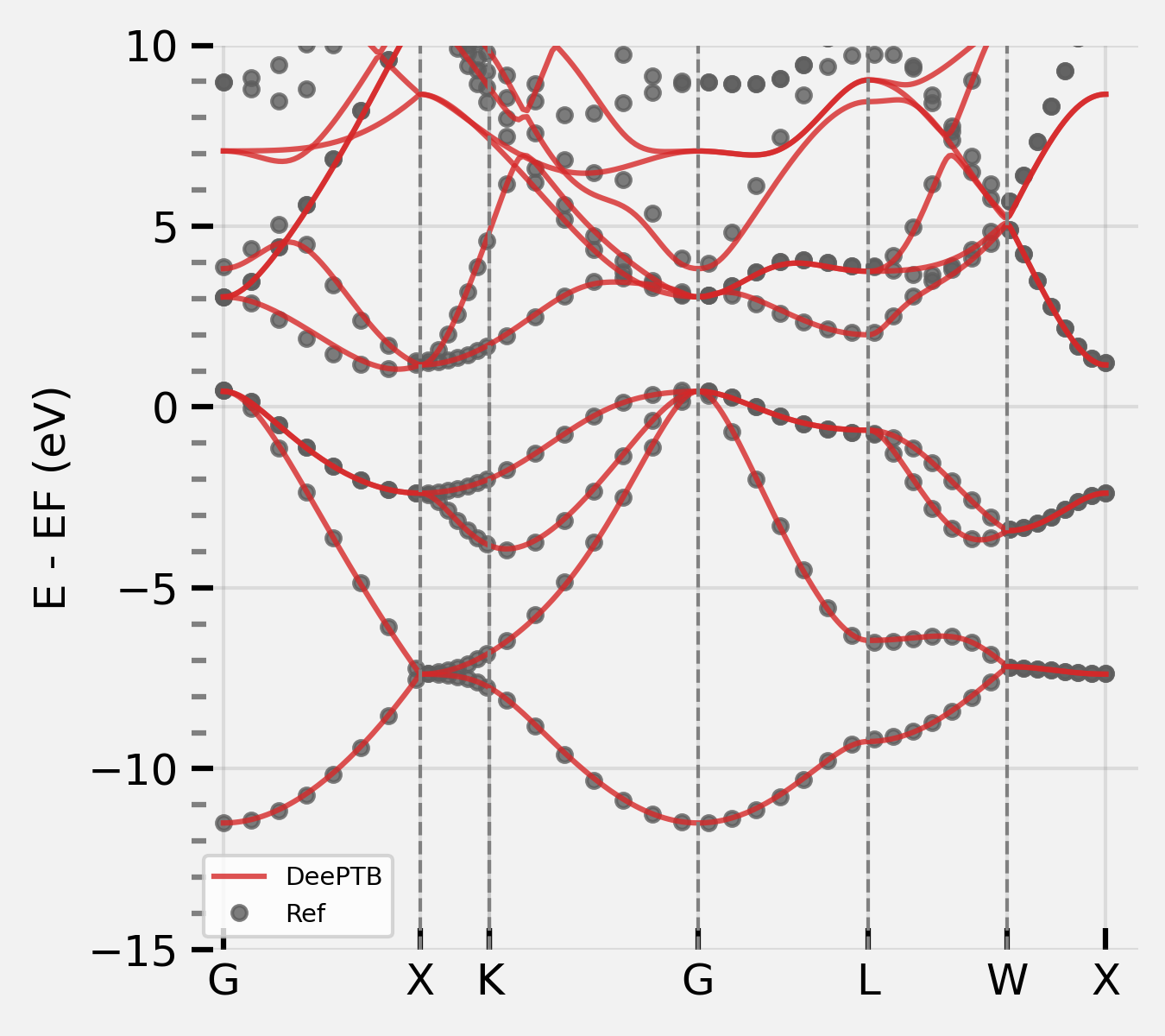
We can plot the converged nnsk model in last step just as in hBN example using band_plot.py script.
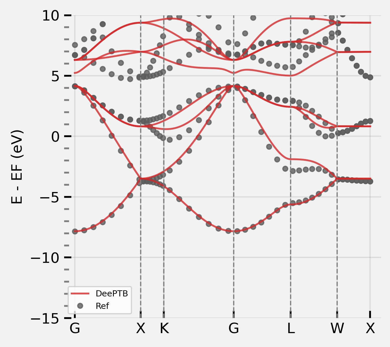
After plotting, we can find that the first fitted model has already captured the shape of the valance bands. However, the conductance band is less accurate since the orbitals 3s and 3p is not complete for the space spanned by the considered valance and conductance band. Therefore we need to include more orbitals in the model.
In DeePTB, users are able to add or remove orbitals by altering the input configuration file. Here we add d* orbital, which can permit us to fit the conductance band essential when calculating excitation properties such as photo-electronics and electronic transport.
First, we add d* in proj_atom_anglr_m of input configuration, which looks like this:
"basis": {
    "Si": ["3s", "3p", "d*"]
    }
Also, we can correct the onsite energies of the TB orbitals using strain method. The nnsk model now looks like:
    "model_options": {
        "nnsk": {
            "onsite": {"method": "strain", "rs":2.5 ,"w":0.3},
            "hopping": {"method": "powerlaw", "rs":2.6, "w": 0.3},
            "freeze": false
        }
    }
Then, we can start training the model with -i/--init-model of our last checkpoint, by running:
dptb train ./input/2-2-1_input.json -i ./nnsk/checkpoint/nnsk.ep495.pth -o ./nnsk_2
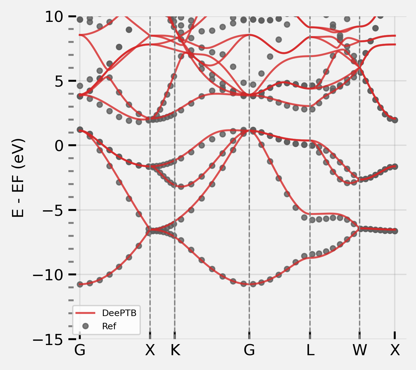
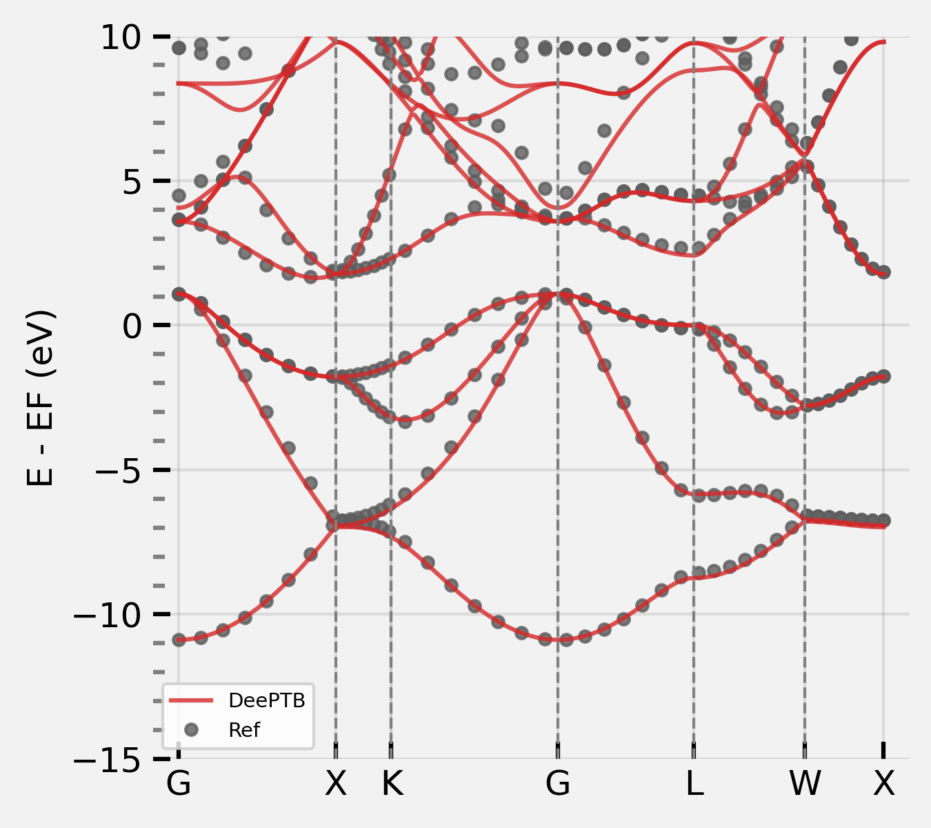
In this way, the parameters in nnsk model corresponding to 3s and 3p orbitals can be reloaded. When convergence is achieved, we can plot the band structure again, which shows that both the valance and conductance bands are fitted well:
Note: In practice, we find that training with the minimal basis set in begin, and then increasing the orbitals gradually is a better choice than directly training with full orbitals from scratch. This procedure can help to reduce the basis size and to improve the training stability.
To further enhance the model, we can enlarge the cutoff range considered, to build a model beyond the first nearest neighbours. The parameter r_max that controls the cutoff radius is set in info.json in the dataset folder.
We now increase the r_max to be larger than the bong-length of the third nearest neighbour, while shorter than the fourth. However, abrupt change in the cutoff will introduce discontinuity in the model training,therefore, a smoothing function is introduced:
and that is controlled by parameters in nnsk keyword in the model_options section of the input file:
rs(angstrom unit): \(r_{skc}\) it controls the cutoff of the decay weight of each bond.w: \(\omega\), it decides the smoothness of the decay.
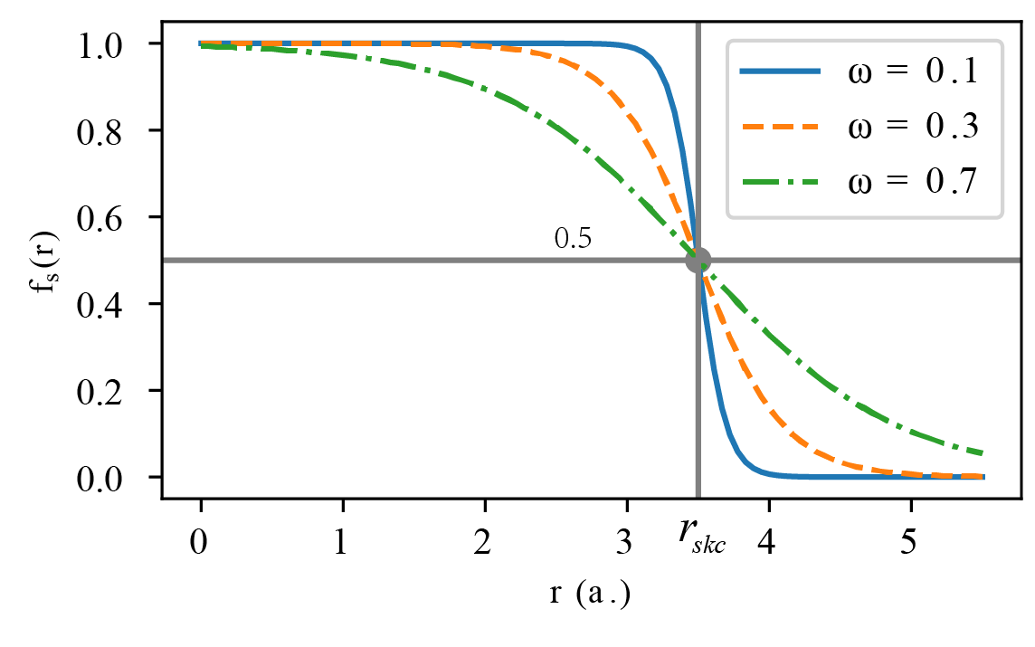
As is shown in the above figure, this smoothing function will decay centred at \(r_{skc}\). According to the smoothness \(\omega\), this function has different smoothness. Here, to take more neighbours’ terms into consideration while retaining the stability of fitting, we first set the \(r_{skc}\) at the first-nearest neighbour distance, this decay function can suppress the newly included second and third neighbour terms, which brings no abrupt changes to the predicted hamiltonians.
Then what is left is pushing \(r_{skc}\) gradually to the value of bond_cutoff. This can be achieved by modifying the parameters in the input configuration and repeating along with training with initialization manually. Alternatively, DeePTB support to push the smooth boundary automatically. We can set the push keyword in nnsk model. push function takes two kinds of input: either push rs by using rs_ths or push w by using w_ths. The rate of the push function is controlled by keyword period. An example of the input model_options for adding neighbors is as follow:
    "model_options": {
        "nnsk": {
            "onsite": {"method": "strain", "rs":2.5 ,"w":0.3},
            "hopping": {"method": "powerlaw", "rs":2.6, "w": 0.3},
            "freeze": false,
            "push": {"rs_thr": 0.024, "period": 15}
        }
    }
DeePTB will push the rs by each step in rs_ths in each period during training. It is recommended to analyse the bond distribution before pushing. The boundary-pushing often takes more training epochs.
We can push the rs first by running:
dptb train ./input/2-2-2_1_input.json -i ./nnsk_2/checkpoint/nnsk.ep501.pth -o ./nnsk_3
After we get the converged model, we can further push the w by running:
dptb train ./input/2-2-2_2_input.json -i ./nnsk_3/checkpoint/nnsk.ep1104.pth -o ./nnsk_4
After adding neighbors, the nnsk model can now fit the bands even better.
2.3 Training the Bond-length Dependent Parameters#
The empirical SK integrals in DeePTB are parameterized by various bond-length dependent functions. This provides the representative power of nnsk model to model the change of electronic structure by atomic distortions. If the user wants to learn the bond-length dependent parameters or would like to add environmental correction to improve the accuracy, or to fit various structures, this step is highly recommended.
The training of Bond-length Dependence parameters will use the dataset of MD snapshots. By modifying the data_options/train/prefix in the input configuration to kpathmd25K/kpathmd100K/kpathmd300K and training the model with initialized checkpoints. The parameters are easily attained. This can be done by running:
dptb train ./input/2-3_1_input.json -i ./nnsk_4/checkpoint/nnsk.ep1501.pth -o ./nnsk_md25
and so on. The bond length dependent model can have a good agreement with the reference bands:
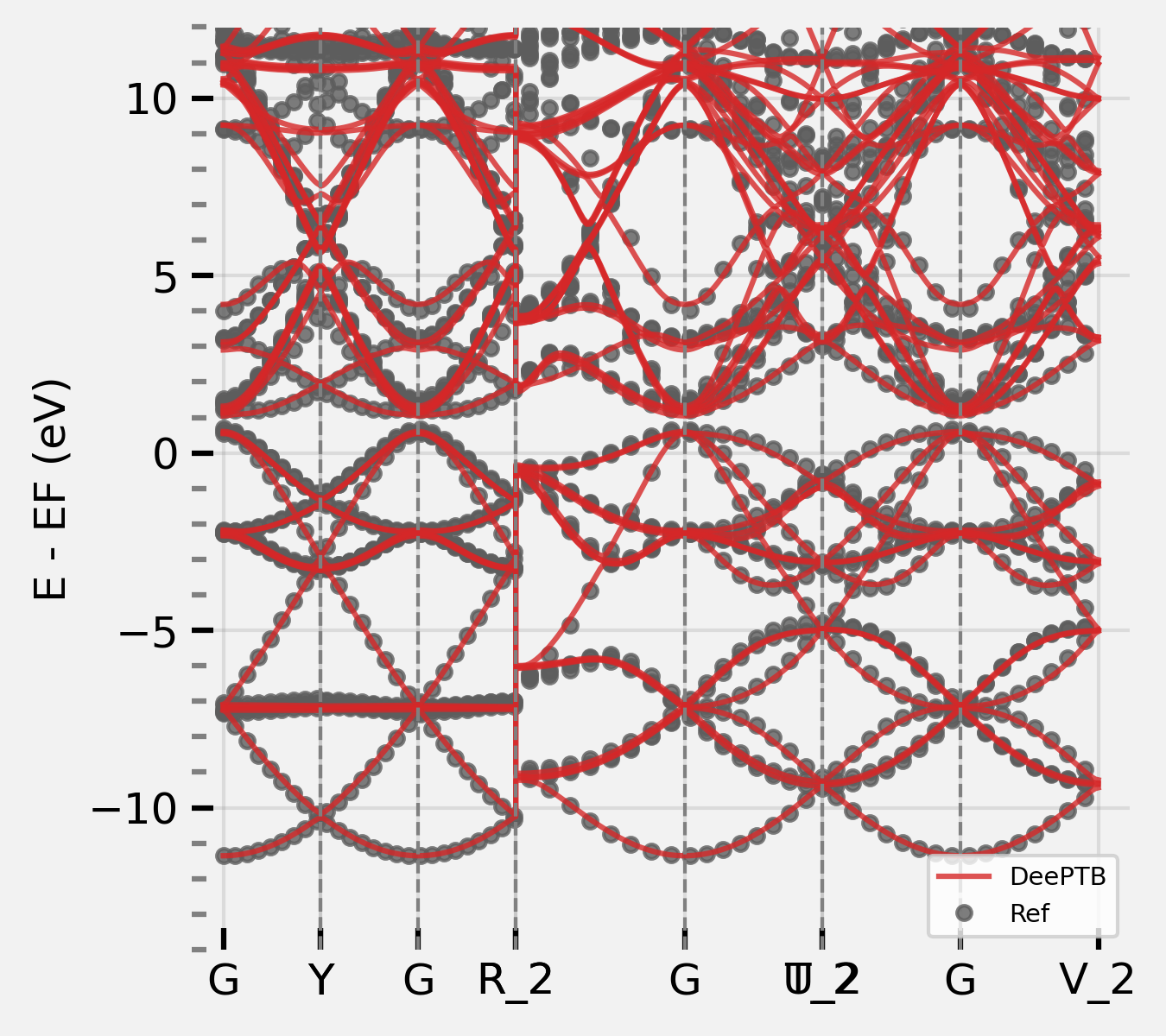
We highly suggest training the model from a low temperature, and the transfer to a higher temperature to improve the fitting stability.
3. Training Deep Learning TB Models with Env. Correction#
DeePTB provides powerful environmental-dependent modelling with symmetry-preserving neural networks. Based on the last step, we can further enhance the power of TB model to overcome the accuracy limit, brought by the two-centre approximation. The environment correction is added by the embedding and prediction part of the model output:
We denote the model that builds the environmental dependence as dptb. To define a dptb model in model_options, we need:
embedding: defines the descriptor of environment.prediction: defines the size of the correction network.nnsk: just as the previousnnskinputs. It is important to set keywordfreezetotruewhen one initializes a newdptbmodel.
With the converged checkpoint in the last step, we can just run:
dptb train ./input/2-4_input.json -i ./nnsk_md25/checkpoint/nnsk.ep43.pth -o ./dptb
We can use the converged model to predict the bandstructure, calculating properties supported by DeePTB, or get the predicted Hamiltonian directly.
Now you know how to train a DeePTB model, congratulations!