Plasticity

Problem definition

Elastoplastic materials, such as metals and engineering alloys, exhibit irreversible deformation behavior characterized by elastic-plastic coupling and path-dependent stress-strain relationships beyond the yield threshold. This example demostrate how to solve the J2 plasticity model [1] using jax_fem, with particular focus on the return mapping algorithm and incremental loading schemes that capture the nonlinear material response under displacement-controlled loading conditions.

For perfect J2-plasticity model [1], we assume that the total strain \(\boldsymbol{\varepsilon}^{n-1}\) and stress \(\boldsymbol{\sigma}^{n-1}\) from the previous loading step are known, and the problem states that find the displacement field \(\boldsymbol{u}^n\) at the current loading step such that

\[-\nabla \cdot \left( \boldsymbol{\sigma}^n(\nabla \boldsymbol{u}^n, \boldsymbol{\varepsilon}^{n-1}, \boldsymbol{\sigma}^{n-1}) \right) = \boldsymbol{b} \quad \text{in } \Omega,\]

\[\boldsymbol{u}^n = \boldsymbol{u}_D \quad \text{on } \Gamma_D,\]

\[\boldsymbol{\sigma}^n \cdot \boldsymbol{n} = \boldsymbol{t} \quad \text{on } \Gamma_N.\]

The weak form gives

\[\int_\Omega \boldsymbol{\sigma}^n : \nabla \boldsymbol{v} \, dx = \int_\Omega \boldsymbol{b} \cdot \boldsymbol{v} \, dx + \int_{\Gamma_N} \boldsymbol{t} \cdot \boldsymbol{v} \, ds.\]

In this example, we consider a displacement-controlled uniaxial tensile loading condition. We assume free traction (\(\boldsymbol{t} = [0,0,0]\)) and ignore body force (\(\boldsymbol{b} = [0,0,0]\)). We assume quasi-static loadings from 0 to 0.1 mm and then unload from 0.1 mm to 0.

The stress \(\boldsymbol{\sigma}^n\) is defined with the following relationships:

\[\boldsymbol{\sigma}_{\text{trial}} = \boldsymbol{\sigma}^{n-1} + \Delta\boldsymbol{\sigma},\]

\[\Delta\boldsymbol{\sigma} = \lambda \text{tr}(\Delta\boldsymbol{\varepsilon})\boldsymbol{I} + 2\mu \Delta\boldsymbol{\varepsilon},\]

\[\Delta\boldsymbol{\varepsilon} = \boldsymbol{\varepsilon}^n - \boldsymbol{\varepsilon}^{n-1} = \frac{1}{2}\left[ \nabla \boldsymbol{u}^n + (\nabla \boldsymbol{u}^n)^T \right] - \boldsymbol{\varepsilon}^{n-1},\]

\[\boldsymbol{s} = \boldsymbol{\sigma}_{\text{trial}} - \frac{1}{3}\text{tr}(\boldsymbol{\sigma}_{\text{trial}})\boldsymbol{I},\]

\[s = \sqrt{\frac{3}{2}\boldsymbol{s}:\boldsymbol{s}},\]

\[f_{\text{yield}} = s - \sigma_{\text{yield}},\]

\[\boldsymbol{\sigma}^n = \boldsymbol{\sigma}_{\text{trial}} - \frac{\boldsymbol{s}}{s}\langle f_{\text{yield}} \rangle_+,\]

where \(\boldsymbol{\sigma}_{\text{trial}}\) is the elastic trial stress, \(\boldsymbol{s}\) is the deviatoric part of \(\boldsymbol{\sigma}_{\text{trial}}\), \(f_{\text{yield}}\) is the yield function, \(\sigma_{\text{yield}}\) is the yield strength, \(\langle x \rangle_+ := \frac{1}{2}(x + |x|)\) is the ramp function, and \(\boldsymbol{\sigma}^n\) is the stress at the current loading step.

Implementation

First, we need to import some useful modules and jax_fem specific modules：

# Import some useful modules.
import jax
import jax.numpy as np
import os
import matplotlib.pyplot as plt


# Import JAX-FEM specific modules.
from jax_fem.problem import Problem
from jax_fem.solver import solver
from jax_fem.utils import save_sol
from jax_fem.generate_mesh import box_mesh_gmsh, get_meshio_cell_type, Mesh

Weak form

In this J2 plasticity example, we use the Laplace Kernel to handle elastoplastic constitutive relations by overriding the get_tensor_map method to define the stress return mapping algorithm that enforces the von Mises yield criterion.

The custom_init() method initializes internal variables self.internal_vars = [self.sigmas_old, self.epsilons_old] to store historical stress and strain states required for path-dependent plasticity computations.

The get_maps() method implements the plasticity algorithms: strain(u_grad) computes the strain tensor from displacement gradients, while stress_return_map(u_grad, sigma_old, epsilon_old) performs the return mapping to project trial stresses back to the yield surface. The update_stress_strain() method advances the internal state variables after each loading increment, ensuring proper tracking of plastic deformation history essential for incremental plasticity formulations.

# Define constitutive relationship.
class Plasticity(Problem):
    # The function 'get_tensor_map' overrides base class method. Generally, JAX-FEM
    # solves -div(f(u_grad,alpha_1,alpha_2,...,alpha_N)) = b. Here, we have
    # f(u_grad,alpha_1,alpha_2,...,alpha_N) = sigma_crt(u_crt_grad, epsilon_old, sigma_old),
    # reflected by the function 'stress_return_map'
    def custom_init(self):
        # Override base class method.
        # Initializing total strain and stress.
        self.fe = self.fes[0]
        self.epsilons_old = np.zeros((len(self.fe.cells), self.fe.num_quads, self.fe.vec, self.dim))
        self.sigmas_old = np.zeros_like(self.epsilons_old)
        self.internal_vars = [self.sigmas_old, self.epsilons_old]

    def get_tensor_map(self):
        # Override base class method.
        _, stress_return_map = self.get_maps()
        return stress_return_map

    def get_maps(self):
        def safe_sqrt(x):
            # np.sqrt is not differentiable at 0
            safe_x = np.where(x > 0., np.sqrt(x), 0.)
            return safe_x

        def safe_divide(x, y):
            return np.where(y == 0., 0., x/y)

        def strain(u_grad):
            epsilon = 0.5*(u_grad + u_grad.T)
            return epsilon

        def stress(epsilon):
            E = 70.e3
            nu = 0.3
            mu = E/(2.*(1. + nu))
            lmbda = E*nu/((1+nu)*(1-2*nu))
            sigma = lmbda*np.trace(epsilon)*np.eye(self.dim) + 2*mu*epsilon
            return sigma

        def stress_return_map(u_grad, sigma_old, epsilon_old):
            sig0 = 250.
            epsilon_crt = strain(u_grad)
            epsilon_inc = epsilon_crt - epsilon_old
            sigma_trial = stress(epsilon_inc) + sigma_old
            s_dev = sigma_trial - 1./self.dim*np.trace(sigma_trial)*np.eye(self.dim)
            s_norm = safe_sqrt(3./2.*np.sum(s_dev*s_dev))
            f_yield = s_norm - sig0
            f_yield_plus = np.where(f_yield > 0., f_yield, 0.)
            sigma = sigma_trial - safe_divide(f_yield_plus*s_dev, s_norm)
            return sigma
        return strain, stress_return_map

    def stress_strain_fns(self):
        strain, stress_return_map = self.get_maps()
        vmap_strain = jax.vmap(jax.vmap(strain))
        vmap_stress_return_map = jax.vmap(jax.vmap(stress_return_map))
        return vmap_strain, vmap_stress_return_map

    def update_stress_strain(self, sol):
        u_grads = self.fe.sol_to_grad(sol)
        vmap_strain, vmap_stress_rm = self.stress_strain_fns()
        self.sigmas_old = vmap_stress_rm(u_grads, self.sigmas_old, self.epsilons_old)
        self.epsilons_old = vmap_strain(u_grads)
        self.internal_vars = [self.sigmas_old, self.epsilons_old]

    def compute_avg_stress(self):
        # For post-processing only: Compute volume averaged stress.
        # (num_cells*num_quads, vec, dim) * (num_cells*num_quads, 1, 1) -> (vec, dim)
        sigma = np.sum(self.sigmas_old.reshape(-1, self.fe.vec, self.dim) * self.fe.JxW.reshape(-1)[:, None, None], 0)
        vol = np.sum(self.fe.JxW)
        avg_sigma = sigma/vol
        return avg_sigma

Mesh

Here we use the first-order hexahedron element HEX8 to discretize the computational domain:

ele_type = 'HEX8'
cell_type = get_meshio_cell_type(ele_type)
data_dir = os.path.join(os.path.dirname(__file__), 'data')

Lx, Ly, Lz = 10., 10., 10.
meshio_mesh = box_mesh_gmsh(Nx=10, Ny=10, Nz=10, Lx=Lx, Ly=Ly, Lz=Lz, data_dir=data_dir, ele_type=ele_type)
mesh = Mesh(meshio_mesh.points, meshio_mesh.cells_dict[cell_type])

Boundary conditions

The boundary conditions implement a displacement-controlled uniaxial tensile test: the bottom surface (\(z=0\)) is fixed with zero displacement constraint dirichlet_val_bottom(point) = 0, while the top surface (\(z=L_z\)) undergoes prescribed displacement loading through get_dirichlet_top(disp). The loading sequence disps defines a loading-unloading cycle from 0 to 0.1 mm followed by unloading back to 0, with both constraints applied to the z-component (vecs = [2, 2]) to simulate the uniaxial tension.

# Define boundary locations.
def top(point):
    return np.isclose(point[2], Lz, atol=1e-5)

def bottom(point):
    return np.isclose(point[2], 0., atol=1e-5)

# Define Dirichlet boundary values.
# We fix the z-component of the displacement field to be zero on the 'bottom'
# side, and control the z-component on the 'top' side.
def dirichlet_val_bottom(point):
    return 0.

def get_dirichlet_top(disp):
    def val_fn(point):
        return disp
    return val_fn

disps = np.hstack((np.linspace(0., 0.1, 11), np.linspace(0.09, 0., 10)))

location_fns = [bottom, top]
value_fns = [dirichlet_val_bottom, get_dirichlet_top(disps[0])]
vecs = [2, 2]

dirichlet_bc_info = [location_fns, vecs, value_fns]

Problem

We have completed all the preliminary preparations for the problem. Then we can proceed to create an instance of our BVP:

problem = Plasticity(mesh, vec=3, dim=3, dirichlet_bc_info=dirichlet_bc_info)

Solver

The defined BVP is solved incrementally using solver() for each displacement step in the loading-unloading cycle. Here, we employ the Newton-Raphson method with PETSc solver, where the internal stress-strain states are updated after each converged solution via problem.update_stress_strain().

avg_stresses = []

for i, disp in enumerate(disps):
    print(f"\nStep {i} in {len(disps)}, disp = {disp}")
    dirichlet_bc_info[-1][-1] = get_dirichlet_top(disp)
    problem.fe.update_Dirichlet_boundary_conditions(dirichlet_bc_info)
    sol_list = solver(problem, solver_options={'petsc_solver': {}})
    problem.update_stress_strain(sol_list[0])
    avg_stress = problem.compute_avg_stress()
    print(avg_stress)
    avg_stresses.append(avg_stress)
    vtk_path = os.path.join(data_dir, f'vtk/u_{i:03d}.vtu')
    save_sol(problem.fe, sol_list[0], vtk_path)

avg_stresses = np.array(avg_stresses)

Postprocessing

The solution can be exported to VTK format files (readable by ParaView and other post-processing software) using jax_fem’s built-in function save_sol:

# Plot the volume-averaged stress versus the vertical displacement of the top surface.
fig = plt.figure(figsize=(10, 8))
plt.plot(disps, avg_stresses[:, 2, 2], color='red', marker='o', markersize=8, linestyle='-')
plt.xlabel(r'Displacement of top surface [mm]', fontsize=20)
plt.ylabel(r'Volume averaged stress (z-z) [MPa]', fontsize=20)
plt.tick_params(labelsize=18)
plt.show()

z-z component of volume-averaged stress versus displacement of the top surface.

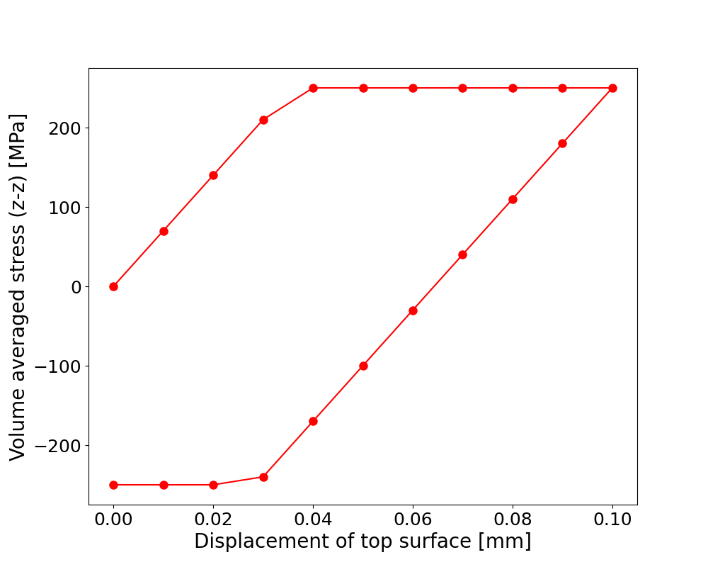
Stress-strain curve.

Please refer to this link to download the source file.

References

1. Simo, Juan C., and Thomas JR Hughes. Computational inelasticity. Vol. 7. Springer Science & Business Media, 2006.

2. Xue, Tianju, et al. “JAX-FEM: A differentiable GPU-accelerated 3D finite element solver for automatic inverse design and mechanistic data science.” Computer Physics Communications (2023): 108802.