Thermal mechanical control#

Problem definition#

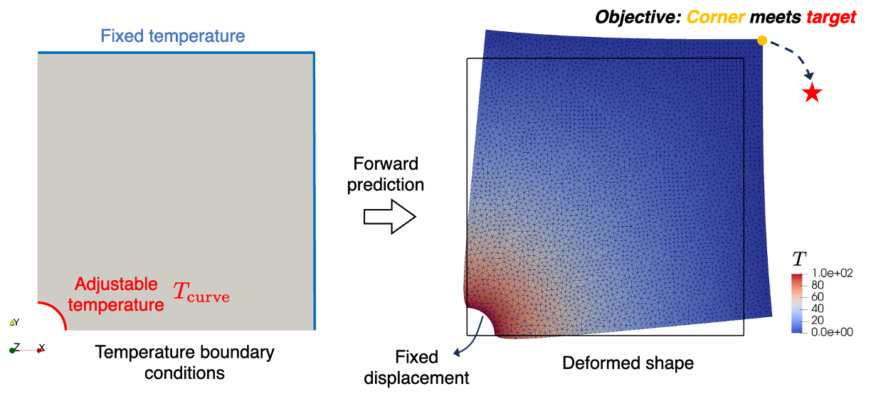
In this example, an inverse problem is considered. The design parameter is the Dirichlet boundary condition. The target of this tutorial is to use JAX-FEM to automatically find the gradient of the objective function with respect to this design variable.

This inverse control problem is to consider thermo-elasticity where a temperature field \(T_{\textrm{curve}}\) applied to a curved boundary is optimized to achieve a desired mechanical deformation. Specifically, the objective is to make the top right corner of a 2D square plate with a circular hole undergo thermal deformation that reaches a prescribed target point.

Governing equations#

The forward thermo-mechanical coupling problem consists of two physics:

1. Steady-state heat conduction:

\[\begin{split}\begin{align*} -\nabla \cdot (k \nabla T) &= 0 &\text{in} \quad \Omega, \\ T &= T_{\textrm{curve}} &\text{on} \quad \Gamma_{D_1, T}, \\ T &= 0 &\text{on} \quad \Gamma_{D_2, T}, \\ k \nabla T \cdot \boldsymbol{n} &= 0 &\text{on} \quad \Gamma_{N, T}, \end{align*}\end{split}\]

where:

\(k\): Thermal conductivity
\(\Omega\): Quarter of a square plate with circular hole (2D)
\(\Gamma_{D_1, T}\): Curved boundary with adjustable temperature
\(\Gamma_{D_2, T}\): Fixed-temperature (\(T=0\)) boundary
\(\Gamma_{N, T}\): Thermally insulated boundary

2. Mechanical equilibrium:

\[\begin{split}\begin{align*} -\nabla \cdot \boldsymbol{\sigma} &= \boldsymbol{0} \quad \text{in} \quad \Omega, \\ \boldsymbol{u} &= \boldsymbol{0} \quad \text{on} \quad \Gamma_{D,\boldsymbol{u}}, \\ \boldsymbol{\sigma} \cdot \boldsymbol{n} &= \boldsymbol{0} \quad \text{on} \quad \Gamma_{N,\boldsymbol{u}}, \end{align*}\end{split}\]

with the thermo-elastic constitutive relation:

\[\begin{split}\begin{align*} \boldsymbol{\sigma} &= \lambda \operatorname{tr}(\boldsymbol{\varepsilon}) \boldsymbol{I} + 2\mu \boldsymbol{\varepsilon} - \kappa T \boldsymbol{I}, \\ \boldsymbol{\varepsilon} &= \frac{1}{2} \left( \nabla \boldsymbol{u} + (\nabla \boldsymbol{u})^T \right), \end{align*}\end{split}\]

where:

\(\boldsymbol{\varepsilon}\): Strain tensor
\(\lambda, \mu\): Lamé parameters (isotropic aluminum)
\(\kappa\): Thermal expansion coefficient
\(T\): Relative temperature change from ambient

Weak form#

Find \(T\) and \(\boldsymbol{u}\) such that for any test functions \(\delta T\) and \(\delta \boldsymbol{u}\):

\[\begin{align*} r(T, \boldsymbol{u}; \delta T, \delta \boldsymbol{u}) = \int_{\Omega} k \nabla T \cdot \nabla \delta T \, \textrm{d}\Omega + \int_{\Omega} \boldsymbol{\sigma} : \nabla \delta\boldsymbol{u} \, \textrm{d}\Omega = 0. \end{align*}\]

This is a one-way coupled system – temperature influences deformation, but deformation does not affect temperature.

Optimization problem#

The inverse control problem is formulated as the following PDE-constrained optimization:

\[\begin{split}\begin{align} \nonumber &\min_{T_\textrm{curve}} \Vert\boldsymbol{u}_{\textrm{corner}} - \boldsymbol{u}_{\textrm{target}}\Vert^2 \\ & \textrm{s.t.} \quad r(T, \boldsymbol{u}; \delta T, \delta \boldsymbol{u})=0, \end{align}\end{split}\]

where \(\boldsymbol{u}_{\textrm{corner}}\) is the displacement at the top-right corner induced by boundary temperature \(T_{\textrm{curve}}\), and \(\boldsymbol{u}_{\textrm{target}}=[0.001, -0.001]\) is the prescribed target displacement.

Implementation#

For the implementation, we first import some necessary modules.

[ ]:

import numpy as onp
import jax
import jax.numpy as np
import os
import meshio
import glob
import sys
import logging

# Import JAX-FEM specific modules.
from jax_fem.problem import Problem
from jax_fem.solver import ad_wrapper
from jax_fem.generate_mesh import get_meshio_cell_type, Mesh, box_mesh_gmsh
from jax_fem import logger

logger.setLevel(logging.INFO)

Weak form#

These global parameters define the fundamental mechanical and thermal properties of the material, which remain constant during the coupled calculation.

[2]:

# Define global parameters (Never to be changed)
T0 = 293. # ambient temperature
E = 70e3
nu = 0.3
mu = E/(2.*(1. + nu))
lmbda = E*nu/((1+nu)*(1-2*nu)) # plane strain
rho = 2700. # density
alpha = 2.31e-5 # thermal expansion coefficient
kappa = alpha*(2*mu + 3*lmbda)
k = 237e-6 # thermal conductivity

The custom_init method initializes two finite element spaces: one for the displacement field (\(\boldsymbol{u}\)) and one for the temperature field (\(T\)).

[ ]:

# Define the coupling problems.
class ThermalMechanical(Problem):
    def custom_init(self):
        self.fe_u = self.fes[0]
        self.fe_T = self.fes[1]

The get_universal_kernel method returns a universal kernel function for computing the weak form. It internally defines strain and stress functions, where the stress calculation considers thermal expansion effects.

[ ]:

    def get_universal_kernel(self):
        def strain(u_grad):
            return 0.5 * (u_grad + u_grad.T)

        def stress(u_grad, T):
            epsilon = 0.5 * (u_grad + u_grad.T)
            sigma = lmbda * np.trace(epsilon) * np.eye(self.dim) + 2 * mu * epsilon - kappa * T * np.eye(self.dim)
            return sigma

The universal_kernel function is the core of the weak form, handling element-level computations. Parameters include the flattened cell solution, coordinates, shape function gradients, Jacobian determinant weights, and test function gradients.

[ ]:

        def universal_kernel(cell_sol_flat, x, cell_shape_grads, cell_JxW, cell_v_grads_JxW):
            # cell_sol_flat: (num_nodes*vec + ...,)
            # x: (num_quads, dim)
            # cell_shape_grads: (num_quads, num_nodes + ..., dim)
            # cell_JxW: (num_vars, num_quads)
            # cell_v_grads_JxW: (num_quads, num_nodes + ..., 1, dim)

            ## Split
            # [(num_nodes, vec), ...]
            cell_sol_list = self.unflatten_fn_dof(cell_sol_flat)
            cell_sol_u, cell_sol_T = cell_sol_list
            cell_shape_grads_list = [cell_shape_grads[:, self.num_nodes_cumsum[i]: self.num_nodes_cumsum[i+1], :]
                                     for i in range(self.num_vars)]
            cell_shape_grads_u, cell_shape_grads_T = cell_shape_grads_list
            cell_v_grads_JxW_list = [cell_v_grads_JxW[:, self.num_nodes_cumsum[i]: self.num_nodes_cumsum[i+1], :, :]
                                     for i in range(self.num_vars)]
            cell_v_grads_JxW_u, cell_v_grads_JxW_T = cell_v_grads_JxW_list
            cell_JxW_u, cell_JxW_T = cell_JxW[0], cell_JxW[1]

            # (1, num_nodes, vec) * (num_quads, num_nodes, 1) -> (num_quads, vec)
            T = np.sum(cell_sol_T[None,:,:] * self.fe_T.shape_vals[:,:,None],axis=1)
            # (num_quads, vec, dim)
            u_grads = np.sum(cell_sol_u[None,:,:,None] * cell_shape_grads_u[:,:,None,:], axis=1)

            ## Handles the term 'k * inner(grad(T_crt), grad(Q)) * dx'
            # (1, num_nodes, vec, 1) * (num_quads, num_nodes, 1, dim) -> (num_quads, num_nodes, vec, dim)
            # -> (num_quads, vec, dim)
            T_grads = np.sum(cell_sol_T[None,:,:,None] * cell_shape_grads_T[:,:,None,:], axis=1)
            # (num_quads, 1, vec, dim) * (num_quads, num_nodes, 1, dim) ->  (num_nodes, vec)
            val3 = np.sum(k * T_grads[:,None,:,:] * cell_v_grads_JxW_T,axis=(0,-1))

            ## Handles the term 'inner(sigma, grad(v)) * dx'
            u_physics = jax.vmap(stress)(u_grads, T)
            # (num_quads, 1, vec, dim) * (num_quads, num_nodes, 1, dim) ->  (num_nodes, vec)
            val4 = np.sum(u_physics[:,None,:,:] * cell_v_grads_JxW_u,axis=(0,-1))

            weak_form = [val4, val3]

            return jax.flatten_util.ravel_pytree(weak_form)[0]

        return universal_kernel

The set_params method allows assigning parameters for the temperature field on the Dirichlet boundary with vals_list.

[ ]:

    def set_params(self, params):
        self.fe_T.vals_list[0] = params

Mesh#

Here we read a mesh input from a local file and use the TRI3 element to discretize the computational domain.

[4]:

meshio_mesh = meshio.read(os.path.join(os.path.dirname(__file__), 'u.vtu'))
ele_type = 'TRI3'
cell_type = get_meshio_cell_type(ele_type)
mesh = Mesh(meshio_mesh.points[:, :2], meshio_mesh.cells_dict[cell_type])

Boundary conditions#

Then we can define the Dirichlet boundary condition. The actual value of \(T\) on the curved boundary will be updated later by the parameter \(\theta\) with the method set_params in the weak form definition above.

[5]:

def right(point):
    return np.isclose(point[0], 1., atol=1e-5)

def top(point):
    return np.isclose(point[1], 1., atol=1e-5)

def hole(point):
    R = 0.1
    return np.isclose(point[0]**2+point[1]**2, R**2, atol=1e-3)

def zero_dirichlet(point):
    return 0.

# The actual hole boundary T will always be updated by the parameters θ, not by this function.
def T_hole(point):
    return 0.

def T_top(point):
    return 0.

def T_right(point):
    return 0.

dirichlet_bc_info_u = [[hole, hole], [0, 1], [zero_dirichlet]*2]
dirichlet_bc_info_T = [[hole, top, right], [0, 0, 0], [T_hole, T_top, T_right]]

Problem#

We have completed all the preliminary preparations for the problem. So, we can proceed to create an instance of our problem.

[ ]:

problem = ThermalMechanical([mesh, mesh], vec=[2, 1], dim=2, ele_type=[ele_type, ele_type], gauss_order=[1, 1],
                                  dirichlet_bc_info=[dirichlet_bc_info_u, dirichlet_bc_info_T])

Solver#

Then we can wrap the forward problem with the function ad_wrapper, which enables efficient gradient computation for our inverse problem.

[7]:

fwd_pred = ad_wrapper(problem)

Then follows the definition of our objective funtion.

[8]:

corner_node_id = 3456 # Top right corner nodal index, obtained from visualization in Paraview
def J(θ):
    u_pred = fwd_pred(θ)
    corner_disp_pred = u_pred[0][corner_node_id]
    corner_disp_goal = np.array([0.001, -0.001])
    error = np.sum(((corner_disp_pred - corner_disp_goal)**2))
    return error

To verify the accuracy of gradients computed using jax.grad, we employ the finite difference method.

[ ]:

hole_boundary_node_inds = problem.fes[1].node_inds_list[0]
hole_boundary_nodes = mesh.points[hole_boundary_node_inds]
num_hole_boundary_nodes = len(hole_boundary_node_inds)
print(f"num_hole_boundary_nodes = {num_hole_boundary_nodes}")

θ_ini = 1e3 *np.ones(num_hole_boundary_nodes)
grad_value = jax.grad(J)(θ_ini)

h = 1e-1
θ_plus = θ_ini.at[10].set((1+h)*θ_ini[10])
θ_minus = θ_ini.at[10].set((1-h)*θ_ini[10])
dx_fd_10 = (J(θ_plus) - J(θ_minus))/(2*h*θ_ini[10])

print(f"\n grad_value[10] = {grad_value[10]}, dx_fd_10 = {dx_fd_10}")

The computation results are shown as follows:

[ ]:

grad_value[10] = 6.960273952781062e-09, dx_fd_10 = 6.960013287569166e-09

Please refer to this link to download the source file.

Thermal mechanical control

Contents

Thermal mechanical control#

Problem definition#

Governing equations#

Weak form#

Optimization problem#

Implementation#

Weak form#

Mesh#

Boundary conditions#

Problem#

Solver#