Traction force identification

Problem definition

In this example, an inverse problem is considered. The design parameter is the Neumann boundary condition. The target of this tutorial is to use JAX-FEM to automatically find the gradient of the objective function with respect to this design variable.

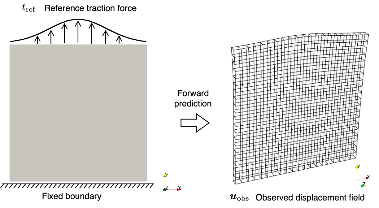
The inverse problem is about identifying an unknown traction force \(\boldsymbol{t}\) on the top boundary of a thin plate, which is fixed at the bottom boundary, based on an observed displacement field \(\boldsymbol{u}_{\textrm{obs}}\). The observed data is generated by solving a forward hyperelasticity problem under a reference traction force \(t_{\textrm{ref}}\).

We consider a typical neo-Hookean solid in the forward problem, whose governing equation of static equilibrium is:

\[\begin{split}\begin{align*} -\nabla \cdot \boldsymbol{P} &= \boldsymbol{0} \quad \text{in} \quad \Omega, \\ \boldsymbol{u} &= \boldsymbol{0} \quad \text{on} \quad \Gamma_D, \\ \boldsymbol{P} \cdot \boldsymbol{n} &= \boldsymbol{t} \quad \text{on} \quad \Gamma_N, \end{align*}\end{split}\]

where \(\boldsymbol{P}\) is the first Piola–Kirchhoff stress tensor, defined through a strain energy density function \(W\):

\[\begin{split}\begin{align*} \boldsymbol{P} &= \frac{\partial W}{\partial \boldsymbol{F}}, \\ \boldsymbol{F} &= \nabla \boldsymbol{u} + \boldsymbol{I}, \\ W(\boldsymbol{F}) &= \frac{G}{2}(J^{-2/3} I_1 - 3) + \frac{\kappa}{2}(J - 1)^2. \end{align*}\end{split}\]

Here:

• \(\boldsymbol{u} : \Omega \rightarrow \mathbb{R}^3\) is the displacement field

• \(\boldsymbol{F}\) is the deformation gradient

• \(J = \det(\boldsymbol{F})\) and \(I_1 = \operatorname{tr}(\boldsymbol{F}^T \boldsymbol{F})\)

• Material parameters:

  • Shear modulus \(G = \frac{E}{2(1+\nu)}\)

  • Bulk modulus \(\kappa = \frac{E}{3(1-2\nu)}\)

  • \(E\) is Young’s modulus, \(\nu\) is Poisson’s ratio

This form of \(W\) is commonly used to model nearly incompressible isotropic elastomers.

Domain and boundary conditions

• \(\Omega = (0,1) \times (0,1) \times (0,0.05)\) (A thin plate)

• \(\Gamma_D = \{(x_1, 0, x_3) \subset \partial \Omega\}\) (Dirichlet boundary)

• \(\Gamma_N = \{(x_1, 1, x_3) \subset \partial \Omega\}\) (Neumann boundary with unknown traction \(\boldsymbol{t}\))

Weak form

Find \(\boldsymbol{u}\) such that for all test functions \(\boldsymbol{v}\),

\[r(\boldsymbol{u}; \boldsymbol{v}) = \int_{\Omega} \boldsymbol{P} : \nabla \boldsymbol{v} \mathrm{d}\Omega - \int_{\Gamma_N} \boldsymbol{t} \cdot \boldsymbol{v} \mathrm{d}\Gamma = 0.\]

Optimization problem

The identification of \(\boldsymbol{t}\) from \(\boldsymbol{u}_{\textrm{obs}}\) is formulated as a PDE-constrained optimization:

\[\begin{split}\begin{aligned} \min_{\boldsymbol{t}} \quad & \int_{\Omega} \| \boldsymbol{u} - \boldsymbol{u}_{\textrm{obs}} \|^2 \mathrm{d}\Omega \\ \text{s.t.} \quad & r(\boldsymbol{u}; \boldsymbol{v}) = 0, \end{aligned}\end{split}\]

which minimizes the mismatch between predicted displacements \(\boldsymbol{u}\) and observed displacements \(\boldsymbol{u}_{\textrm{obs}}\).

Implementation

For the implementation, we first import some necessary modules.

import numpy as onp
import jax
import jax.numpy as np
import os
import matplotlib.pyplot as plt

# Import JAX-FEM specific modules.
from jax_fem.problem import Problem
from jax_fem.solver import ad_wrapper
from jax_fem.generate_mesh import get_meshio_cell_type, Mesh, box_mesh_gmsh

Weak form

The definition of the hyperelastic problem is shown as follows. In this problem, the parameter to be optimized is the value of Neumann boundary condition. We use the internal variable on boundary self.internal_vars_surfaces in the method set_params to pass the value of Neumann boundary condition to get_surface_maps. Generally, we can also assign values of multiple Neumann boundary condtions in self.internal_vars_surfaces.

class HyperElasticity(Problem):
    def custom_init(self):
        self.fe = self.fes[0]

    def get_tensor_map(self):
        def psi(F):
            E = 1e6
            nu = 0.3
            mu = E/(2.*(1. + nu))
            kappa = E/(3.*(1. - 2.*nu))
            J = np.linalg.det(F)
            Jinv = J**(-2./3.)
            I1 = np.trace(F.T @ F)
            energy = (mu/2.)*(Jinv*I1 - 3.) + (kappa/2.) * (J - 1.)**2.
            return energy
        P_fn = jax.grad(psi)

        def first_PK_stress(u_grad):
            I = np.eye(self.dim)
            F = u_grad + I
            P = P_fn(F)
            return P
        return first_PK_stress

    def get_surface_maps(self):
        def surface_map(u, x, load_value):
            return np.array([0., -load_value, 0.])
        return [surface_map]

    def set_params(self, params):
        surface_params = params
        # Generally, [[surface1_params1, surface1_params2, ...], [surface2_params1, surface2_params2, ...], ...]
        self.internal_vars_surfaces = [[surface_params]]

Mesh

Here we use the first-order hexahedron element HEX8 to discretize the computational domain:

# Specify mesh-related information (first-order hexahedron element).
output_dir = os.path.join(os.path.dirname(__file__), f'output')
fwd_dir = os.path.join(output_dir, 'forward')
os.makedirs(output_dir, exist_ok=True)

ele_type = 'HEX8'
cell_type = get_meshio_cell_type(ele_type)
Lx, Ly, Lz = 1., 1., 0.05
meshio_mesh = box_mesh_gmsh(Nx=20, Ny=20, Nz=1, domain_x=Lx, domain_y=Ly, domain_z=Lz, data_dir=fwd_dir, ele_type=ele_type)
mesh = Mesh(meshio_mesh.points, meshio_mesh.cells_dict[cell_type])

Boundary conditions

The Dirichlet boundary condition is defined on the bottom side of the computational domain. And the Neumann boundary condtion is defined on the top side.

def zero_dirichlet_val(point):
    return 0.

def bottom(point):
    return np.isclose(point[1], 0., atol=1e-5)

def top(point):
    return np.isclose(point[1], Ly, atol=1e-5)

dirichlet_bc_info = [[bottom]*3, [0, 1, 2], [zero_dirichlet_val]*3]
location_fns = [top]

Problem

We have completed all the preliminary preparations for the problem. So, we can proceed to create an instance of our problem.

problem = HyperElasticity(mesh, vec=3, dim=3, ele_type=ele_type, dirichlet_bc_info=dirichlet_bc_info, location_fns=location_fns)

Solver

Then we can wrap the forward problem with the function ad_wrapper, which enables efficient gradient computation for our inverse problem.

fwd_pred = ad_wrapper(problem)

To generate the observed solution field \(\boldsymbol{u}_{\textrm{obs}}\), we define a reference traction \(t_{\textrm{ref}}\) as:

\[t_{\textrm{ref}}(\boldsymbol{x})=10^5\,\textrm{exp}\big(-(x_1-0.5)^2/0.08 \big)\]

The observed solution \(\boldsymbol{u}_{\textrm{obs}}\) is then obtained by substituting \(t_{\textrm{ref}}\) into the forward problem.

# (num_selected_faces, num_face_quads, dim)
surface_quad_points = problem.physical_surface_quad_points[0]
traction_true = 1e5*np.exp(-(np.power(surface_quad_points[:, :, 0] - Lx/2., 2)) / (2.*(Lx/5.)**2))
sol_list_true = fwd_pred(traction_true)

Then we can define the objective funtion, which is the l2 error between predicted solution \(\boldsymbol{u}\) and observed data \(\boldsymbol{u}_{\textrm{obs}}\).

def compute_l2_error(problem, sol_list_pred, sol_list_true):
    u_pred_quad = problem.fes[0].convert_from_dof_to_quad(sol_list_pred[0]) # (num_cells, num_quads, vec)
    u_true_quad = problem.fes[0].convert_from_dof_to_quad(sol_list_true[0]) # (num_cells, num_quads, vec)
    l2_error = np.sum((u_pred_quad - u_true_quad)**2 * problem.fes[0].JxW[:, :, None])
    return l2_error

def J(θ):
    sol_list_pred = fwd_pred(θ)
    l2_error = compute_l2_error(problem, sol_list_pred, sol_list_true)
    return l2_error

To verify the accuracy of gradients computed using jax.grad, we employ the finite difference method.

traction_ini = 1e5*np.ones_like(surface_quad_points)[:, :, 0]
grad_value = jax.grad(J)(traction_ini)

h = 1e-5
traction_plus = traction_ini.at[10, 3].set((1+h)*traction_ini[10, 3])
traction_minus = traction_ini.at[10, 3].set((1-h)*traction_ini[10, 3])
dx_fd_1003 = (J(traction_plus) - J(traction_minus))/(2*h*traction_ini[10, 3])

print(f"\n grad_value[10, 3] = {grad_value[10, 3]}, dx_fd_1003 = {dx_fd_1003}")

The computation results are shown as follows:

grad_value[10, 3] = 2.819967388157955e-11, dx_fd_1003 = 2.8199675084742033e-11

Please refer to this link to download the source file.